The first post in this series is here. The previous post in this series is here. The next post in this series is here.
To add a bit of an explanatory touch to our texts, we started a mini-series, in which we explain scientific foundations of neural networks technologies for those, who have little prior knowledge. The purpose is to really show you what is going on behind the curtain. Even if you are completely new to this field!
Those, who are into the latest language tech innovations, very likely came across the notion of a neural network. You probably also heard of a machine and deep learning. Maybe you are even considering the larger deployment of these technologies in your organization?
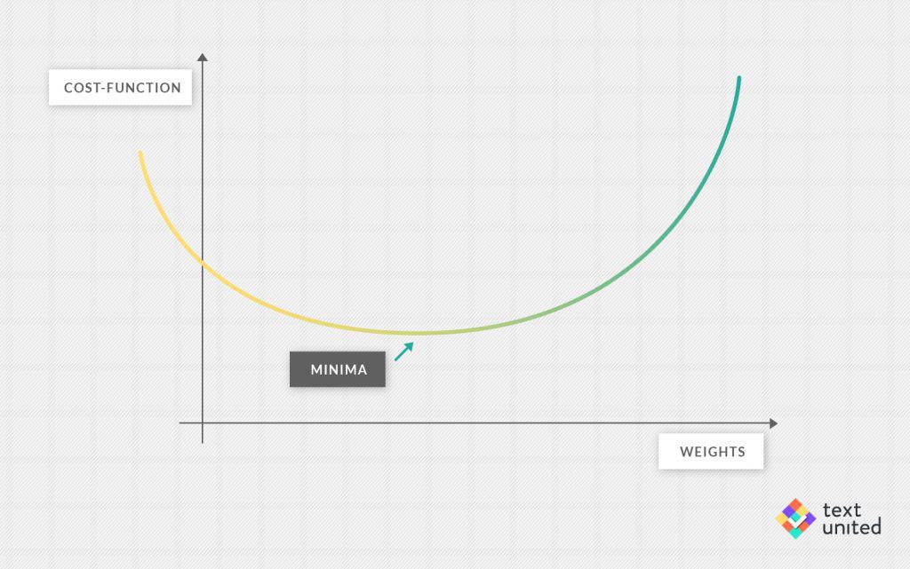
We have already explained what a neuron is and how it makes connections in Part One and what does the neural network really ‘do’ in Part Two. In Part Three of our series we took a look at how machines ‘learn’ and today, we will continue to explain the notion of a cost function today. To remind you, the cost-function measures how well our neural network is performing. A small cost-function means the network does a good job, while a large one means that it does a bad job.
Now It Is Important To View a Neural Network as Something Dynamic Rather Than Static.
For example, you might think that increasing a particular weight might improve performance. But how do you check it? You look just at the cost-function. If the cost-function will go down, then increasing that weight really helped. There is a systematic way for this procedure called ‘gradient descent’. You might remember this from school when you were asked to find the minimum of a function.
For easy examples, this is done by setting the first derivative to zero. For the kind of problems encountered in machine learning, this is however infeasible. The problem is the dimensionality or the number of parameters. Remember there are about 12.000 weights in our neural network!
Local Minima
To explain what is done here, let’s use a pleasant analogy. Imagine you are in the mountains and there is a very thick fog. You want to get to the valley, but you cannot see for more than 10 meters. Where do you go? Well, the best thing to do seems to be going in the direction of the steepest descent. That way, you will hopefully find your way down. In the worst case, you might get stuck in a so-called ‘local minima’. In our example that would be at the bottom of a dried out lake somewhere high in the mountains, where it would seem that it goes up in any direction. This is indeed a problem for machine learning, however, such local minima are usually still good enough.
You can think of the cost-function as being the landscape and the 12.000 parameters corresponding to the location. By randomly initializing the weights you will essentially start from a random point on the landscape. Now, remember, you want to minimize the cost-function, which is just equivalent to finding the valley. But how do you find the direction of steepest descent? Well, you need to compute the gradient of the cost function, and the right direction would be just minus the gradient (you can think of a gradient just as an ordinary derivative of a function).
This process is called ‘learning’ and is often computationally expensive. Various techniques have been developed to improve it, like stochastic gradient descent or regularization. In fact, there is a whole separate field of mathematics called ‘optimization’ which is concerned with finding the best algorithms to do the job. But details do not matter for our purposes. The main takeaway message is that there is a way to iteratively tweak the 12.000 weights, so as to minimize the cost function.
Measurement of Accuracy
But recall that the cost-function measures the error of our neural network. By minimizing it, we have eliminated a lot of these errors. The hope is that our neural network will be quite good and be doing the thing we have taught it to do. In our case, the task is the classification of handwritten digits and with our simple setup, one can achieve accuracies above 95 percent. That is quite impressive. Admittedly, the task is rather simple. As you can imagine, things get a lot trickier if you want to do machine translation and there is a lot of active research in that direction.
It might seem that the only thing that we need to consider is the cost-function and how small it is. But there is a risk that instead of learning to recognize handwritten digits, our network just learns the training data by heart. This can happen if there are too many adjustable parameters or if the training size is too small.
If this happens, the network will perform very well on the training data, but will not be able to generalize to new data. The term for this phenomenon is ‘overfitting’. It must be avoided and again many techniques have been developed like regularization or dropout to counter this problem. Either way, if you want to measure the accuracy of a neural network, you must not use the training data but rather so-called, ‘test data’ which has not been used for learning.
In the next part, we will get the first glimpse of natural language processing and its relation to neural networks.
Stay tuned!