
The first post in this series is here. The previous post in this series is here. The next post in this series is here.
Welcome back to the series where we explain scientific foundations of neural network technologies to outline what a Neural Network actually is, then dive into their use of natural language processing and consecutively, neural machine translation. The purpose of all that is to really show you what is going on behind the curtain.
In Part Six, we discussed the success rate of a neural network.
Today we will take a closer look at word vectors and vector spaces. You might remember them from school and think of them as an arrow in the plane (or in 3-dimensional space). The usual notation is that of a column of real numbers, but for our purposes, it is easier just to write it as a row vector, e.g. (1,2) :
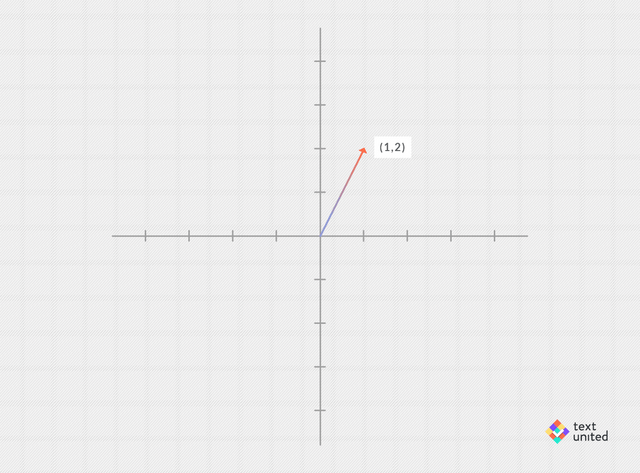
You might consider vectors in higher dimensions, that is, consisting of many real numbers like (1.2, 0, -5.3, 2). In fact, word vectors in general can have hundreds of dimensions! As scary, as that sounds, the math turns out to be exactly the same as in the case of the plane. So we will stick to vectors having just two components, to keep things simple. The wonderful thing is that you can add them. You do this componentwise. That means you add together each component separately, for example
(1,2) + (3,1) = (4,3)
This can be visualized nicely:

In the same spirit, one can subtract two vectors, e.g. (1,2) – (3,1) = (-2,1):

What’s more, you can multiply any of them by a real number, for example,
2*(1,2) = (2,4)
This just corresponds to scaling (in this case by a factor of 2). As real numbers are sometimes called scalars, this operation is called ‘scalar product’ (product is just another word for multiplication).

Can you also multiply two vectors? The answer is yes, but what you get is only a number. It works by multiplying each pair of components and then summing up. Hence,
(1,2)*(3,4) = 1*3 + 2*4 = 3 + 8 = 11
This product is called ‘inner product’. Now, what is the geometric interpretation? Well, let’s look at a vector multiplied with itself, for example (3,4). We have
(3,4)*(3,4) = 3*3 + 4*4 = 9+ 16 = 25
Taking the square root gives 5, which is just the length of the vector (3,4) (use Pythagoras theorem if you are not convinced). So if a vector is multiplied by itself, the result is the length squared. What about
(3,4)*(-4,3)?
Note, we have switched the entries and added a minus sign in the second vector. I will let you do this on your own. The result is a 0.
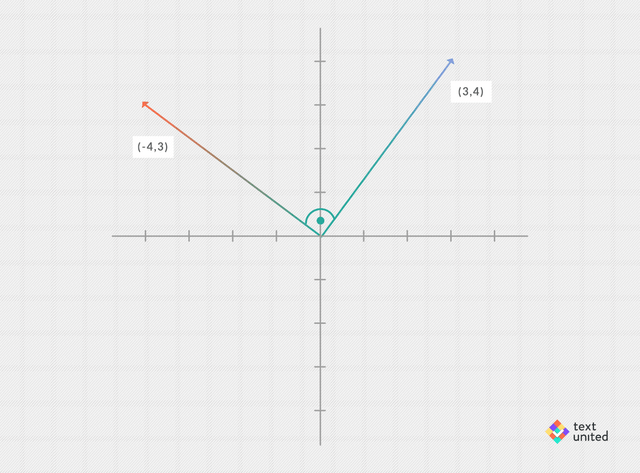
You probably notice that there is an angle of 90 degrees between both vectors. That’s no coincidence. In fact, the inner product of two vectors is 0 precisely when they are 90 degrees apart. That’s a crucial geometric insight captured in algebra. For two arbitrary vectors, one can think of the inner product as the product of their lengths times a number, which depends only on the angle between the two vectors.
It turns out that this number is just the cosine of the angle (don’t worry if you don’t know what the cosine is). From the considerations above it follows that
cos(0°) = 1 and cos(90°) = 0
In general, one can use the cosine-function of the angle or the inner product to measure how ‘close’ two vectors are to each other. It gives us a concept of a ‘distance’. And as we will see, this will allow us to capture the notion of two words being close to one another by looking at the distance of their vectors. It is a good moment to sum up what we have learned about vectors so far and give a preview of what we will do next:
• Vector addition: two vectors can be added
• Vector subtraction: two vectors can be subtracted
• Scalar product: a vector can be multiplied by a real number
• Inner product: two vectors can be multiplied
• Angle: two vectors define an angle between them
The last two points can be used to define a distance between vectors. In the case of the inner product one gets the so-called ‘Euclidean distance’ (it is a bit more complicated then just taking the inner product of the two vectors in question, but we do not need to know how it is done exactly). With the angle one can define something similar to a distance, where one is ignoring the length of the vectors and only focuses on the directions. Either way, from now on we will take it for granted that we have a quantitative notion of distance and so we will be able to say for example that vector y is closer to vector x, then to vector z.
Let me again emphasize that this works in any dimension and that the computation complexity is linear in the dimension, which implies that any computer can handle word vectors containing, say 1000 entries (though the actual process of learning word vectors scales differently). You might ask yourself what all this fuss is about. It turns out that a lot of semantics and syntactics is captured in the linear structure of words vectors. To explain this, we will first need a compact notation relating words with their vector representations. We will simply write
vec(‘x’) for the word vector of the word ‘x’
Hence, for example,
the word vector of ‘tree’ is vec(‘tree’)
which written down would give us just a sequence of say 100 real numbers:
vec(‘tree’) = (0.3, 2.1, 1, -2.3, …)
Now let me ask you this. What is
vec(‘Germany’) + vec(‘capital’)
equal to? Probably, the first word that came to your mind is ‘Berlin’.Unfortunately, the above expression will never be exactly
vec(‘Berlin’)
But remember, we can talk in a quantitative manner about two vectors being close to one another. So we might look for the word vector closest to
vec(‘Germany’) + vec(‘capital’)
And here the magic happens. Its indeed vec(‘Berlin’):

But there is more! One can also consider analogy reasoning tasks.
‘Madrid’ is to ‘Spain’ as ‘x’ is to ‘France’
How does one capture relations between two words like a country and its capital, in the language of vectors? Maybe you should pause and think about it. Scroll up and look at the graphical representations of different vector operations. What do you think? The right answer is: subtraction. The picture below should clear things up:

We have visualized vectors not as arrows but rather as points, which are placed where the arrowheads would normally be. The two arrows represent vectors
vec(‘Madrid’)-vec(‘Spain’) and vec(‘Paris’)-vec(‘France’)
Pretending we don’t know yet that ‘x’ should be Paris, we postulate from the picture above, that both arrows are equal, and hence
vec(‘Madrid’) – vec(‘Spain’) = vec(‘x’) – vec(‘France’)
Using elementary algebra (taking vec(‘France’) to the other side) this is equivalent to
vec(‘Madrid’) – vec(‘Spain’) + vec(‘France’) = vec(‘x’)
We cannot hope for both sides being equal but we can look for the ‘x’, such that vec(‘x’) is closest to the left-hand side. We happily find out that this word is indeed ‘Paris’. It is worth taking a moment and appreciating how amazing this it. We can teach a computer to embed our vocabulary into high-dimensional spaces, such that semantic relations are captured by the linear structure. We are talking here about literally doing high school algebra (addition, subtraction, multiplication) with words. The only caveat is that the spaces are highly dimensional.
As mentioned before, that is not a serious problem, as modern computers can easily handle this complexity. Vector spaces are universal and useful objects, as they have a lot of structure, while still being very simple. Word vector representations are just one example of many and of how they spaces can be applied in science and technology. That one can use vector addition and subtraction to get meaningful results was first discovered by Mikolov et al. and outlined in the papers ‘Distributed Representations of Words and Phrases and their Compositionality’ and ‘Efficient Estimation of Word Representations in Vector Space’ dating back to 2013. In fact, the above examples are taken directly from those papers. The researchers used a model called ‘Word2vec’, which is an improvement of the model I described in the last blog. We’ll explain more about this next time.
Note that while 2013 seems fairly recent, a lot has been going on since then in the field of neural networks, and so the analogy tasks that machines can perform today are a lot more sophisticated than the rather simple ones given above. Finally, I will give you something to ponder about. Vocabularies can be nicely embedded into vector spaces. Does this embedding depend on the language? From the point of view of neural translation, the hope is that such embeddings would be in some sense universal.
We will explore this question in the upcoming blog entries.